TThe Apple® Gazette

Plotting Polar Graphs With The Apple II
Marvin L. De Jong
The School of the Ozarks
Pt. Lookout, MO 65726
You do not need long programs to make a computer perform a useful task in teaching mathematics. One of the more arduous tasks in trigonometry or analytic geometry is graphing functions in polar coordinates. For many polar curves, this task takes a lot of time, and not much learning takes place. On the other hand, it is an ideal task for the computer, the program to plot a polar graph is easily understood by the students, and it gives them a tool with which they can experiment with many graphs. Program 1 shows the simplest possible version. We shall discuss it shortly, but first here is a brief explanation of what we are trying to accomplish.
Suppose we have a relation between R, the distance from a point called the pole, and θ (Greek symbol theta), the angle measured counterclockwise from the polar axis. The pole is analogous to the origin in X-Y Cartesian coordinates, and the polar axis lies along the X-axis. The relation between R and θ is usually described by an equation of the form
R = F(θ).
The equation
R = 90 * SIN(2 * θ)
is one example. Refer to Figure 1 for an illustration of some of these concepts, including a graph of the equation R = 90*SIN(2*θ), called a four-leaved rose.
The key to using a computer to graph polar coordinates is the transformation formulas
X = R * COS(θ)
Y = R * SIN(θ)
and, of course, the computer's ability to perform a PLOT X, Y instruction.
A "bare bones" approach to plotting polar graphs is given in Program 1. The student inputs the starting angle and the angle at which the graph is to end. These angles are in degrees. Line 30 initializes the HIRES mode with text on the lower part of the screen of the video monitor. Line 60 converts the angle to radians (pi radians = 180°).
Line 70 in Program 1 is the equation to be graphed. The entire program may be left unchanged while line 70 is modified to graph a large variety of polar functions.
Figure 1. A Four-Leaved Rose. R = 90*SIN(2*THETA)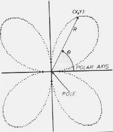
Line 90 and 100 convert the polar coordinates (R,θ) to X-Y coordinates. Note that since the origin of the Apple II coordinate system is in the upper left-hand corner of the screen, we have translated it so the origin of our coordinate system is at (85,85). Furthermore, since Y is positive downward on the Apple, and we would prefer the more traditional "Y positive upward" convention, we use a negative sign in the Y-transformation equation. The results are plotted with the instruction on line 120. The instruction on line 130 increments the angle by one degree. Points will be continued to be plotted until the angle exceeds the ending angle. The student can watch the points being plotted and see the corresponding R and 0 values printed underneath the graph.
Figure 2:A Nineteen-Leaved Rose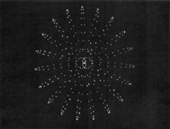
A photograph of the screen of the video monitor after the graph R = 85*SIN (19*THETA) was plotted is shown in Figure 2. Notice that different X and Y scale factors on the screen produce a slight distortion that is not important as far as the present application is concerned.
Of course, it is always possible to add a few bells and whistles. Program 2 represents a few non-essential, but nice, additions to the first program. The coordinate axes are drawn and the X and Y values are rounded to their nearest integer values before plotting. Also, we have made use of the entire screen with the HGR2 instruction on line 30. The scale of the graph was reduced so that we could plot the finished result on our little printer. If you are using a video monitor or a large printer, then you will want to keep the scale as large as possible (replace all the 80's with 90's).
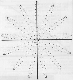
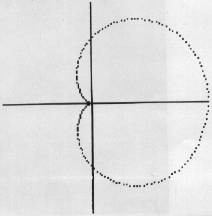
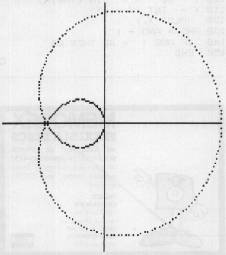
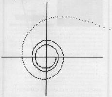
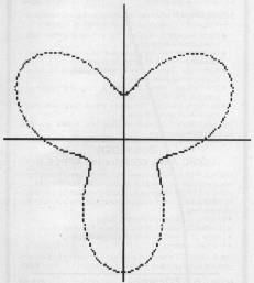
Some of our results are given in the figures that follow. In Figure 3 we show a graph of R = 80*SIN(3*THETA) a three-leaved rose. Figure 4 is a graph of a 13-leaved rose, R = 80*SIN(13* THETA). The cardioid R = 40*(1 + COS(THETA)) is illustrated in Figure 5. Figure 6 is the famous Spiral of Archimedes, R = 6*THETA. Figure 7 is similar, but not identical to the Limacon of Pascal. We chose R = 80*COS(THETA/3) for this figure. Figure 8 illustrates the Litus described by the equation R = 25*(2 + SIN(3*THETA)). Figure 9 has no name, but its equation is R = 25*(2 + SIN(3*THETA)).
Finding where two polar curves intersect is sometimes difficult. If you have a printer you can simply graph the polar curves, overlay their graphs, and find approximate points of intersection.
Figure 3. A Three-Leaved Rose. R = 80*SIN(3*THETA)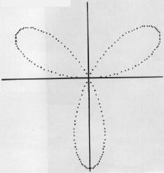
Students seem to enjoy working with these programs. They are simple enough so the students can modify the various parameters rather easily, giving them a chance to experiment freely. At the very least, the programs release them from the drudgery of plotting points by hand.
Figure 6. Spiral of Archimedes with R = 6* THETA. R = 6*THETA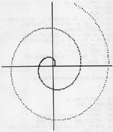
COMPUTE! The Resource
Program 1. A Simple Program to Graph Polar Functions
← LIST
10 INPUT AA, AB
20 ANG = AA
30 HGR
60 THETA = 3.1415926 * ANG / 180
70 R = 85 * SIN (2 * THETA)
80 PRINT R, ANG
90 X = 85 + R * COS (THETA)
100 Y = 85 - R * SIN (THETA)
120 HPLOT X, Y
130 ANG = ANG + 1
140 IF ANG < = AB THEN 60
150 END
Program 2. An Elaboration of Program 1.
← LIST
10 INPUT AA, AB
20 ANG = AA
30 HGR2
40 HPLOT 1,80 TO 160,80
50 HPLOT 80,1 TO 80,160
60 THETA = 3.1415926 * ANG / 180
70 R = 80 * SIN (3 * THETA)
80 X = 80 + R * COS (THETA)
90 X = INT (X + .5)
100 Y = 80 - R * SIN (THETA)
110 Y = INT (Y + .5)
120 HPLOT X, Y
130 ANG = ANG + 1
140 IF ANG < = AB THEN 60
150 END